


My PhD student, Congzheng Liu (co-supervised with Adam Letchford) has written a paper, entitled “Newsvendor Problems: An Integrated Method for Estimation and Optimisation“. This paper has recently been published in EJOR. In this paper we build upon the existing Ban & Rudin (2019) approach for newsvendor problem, showing that in case of the linear model, it becomes equivalent to quantile regression. We then extend it for the non-linear newsvendor problems, testing it on simulated and real life data. In order to understand what specifically we propose, we need to discuss the typical process in case of newsvendor problem.
Newsvendor is a class of problems, where the product can only be sold one day, after which it goes to waste. So this is appropriate, for example, for perishable products in retail. Typically, in this situation we would have historical demand of sales of our product \(y_t\) and we would try forecasting it using regression / ETS / ARIMA or any other model. After doing that and obtaining the estimates of parameters, we would produce a quantile of assumed distribution, which then tells us how much to order (\(q_t\)). If we order more than needed, we will have holding costs. In the opposite case, we will have shortage costs. Based on these costs and the price of product, we can find the optimal order, that will give the maximum profit.
As you can already spot, the forecasting stage is detached from the optimisation one in this situation. The idea of the proposed integrated approach (IMEO) is simple: instead of optimising the model via MSE or any other conventional loss and then solving the optimisation problem, we could estimate the model via maximisation of the specific profit function, thus obtaining the required orders directly. This is not a new idea on its own, but using profit function rather than the cost (as Ban & Rudin, 2019 did) allows applying IMEO to wider set of problems.
For example, if we know the price of the product \(p\), the costs for production \(v\), holding \(c_h\) and shortage costs \(c_s\), we can then calculate profit as (for a linear newsvendor problem):
\begin{equation}
\pi(q_t,y_t)=
\begin{cases}
p y_t -v q_t -c_h (q_t -y_t),& \text{for } q_t \geq y_t\\
p q_t -v q_t -c_s (y_t -q_t),& \text{for } q_t< y_t,
\end{cases}
\end{equation}
where \(q_t\) is the order quantity and \(y_t\) is the actual sales. This profit function can be used for the estimation of a model of your choosing. Congzheng has written a separate R code for the experiments for the paper. Inspired by his example, I have implemented custom losses in alm() and adam() functions from respective greybox and smooth packages for R. At the moment, only the regression model works properly with custom losses – ETS / ARIMA need additional modifications, which we will hopefully resolve in the next paper. So, here is an example with linear newsvendor problem and alm():
# Generate artificial data
x1 <- rnorm(100,100,10)
x2 <- rbinom(100,2,0.05)
y <- 10 + 1.5*x1 + 5*x2 + rnorm(100,0,10)
ourData <- cbind(y=y,x1=x1,x2=x2)

# Define price and costs
price <- 50
costBasic <- 5
costShort <- 15
costHold <- 1

# Define profit function for the linear case
lossProfit <- function(actual, fitted, B, xreg){
    # Minus sign is needed here, because we need to minimise the loss
    profit <- -ifelse(actual >= fitted,
                     (price - costBasic) * fitted - costShort * (actual - fitted),
                     price * actual - costBasic * fitted - costHold * (fitted - actual));
    return(sum(profit));
}

# Estimate the model
model1 <- alm(y~x1+x2, ourData, loss=lossProfit)

# Print summary of the model
summary(model1, bootstrap=TRUE)
Response variable: y
Distribution used in the estimation: Normal
Loss function used in estimation: custom
Bootstrap was used for the estimation of uncertainty of parameters
Coefficients:
            Estimate Std. Error Lower 2.5% Upper 97.5%
(Intercept)  36.5177    14.2840     2.7783     51.4844 *
x1            1.3622     0.1622     1.1909      1.7528 *
x2            3.3423     2.7810    -6.5997      5.9101

Error standard deviation: 17.2266
Sample size: 100
Number of estimated parameters: 3
Number of degrees of freedom: 97
The resulting model is easy to work with: it provides meaningful parameters, showing how on average the order should change if a variable changes by one. For example, we see that with the increase of the variable x1, the orders should change on average by 1.36.
Note that in this specific case, as shown in our paper, the model would be equivalent to the quantile regression, estimated for the quantile \(\left( \frac{c_u}{c_o+c_u} \right)\), where \(c_u= p-v+c_s\) is the "underage" cost and \(c_o = v+c_h\) is the "overage" cost. In our example it corresponds to approximately 0.9091 quantile. We can compare the output of this model with the one from the quantile regression in alm (which is estimated as an Asymmetric Laplace model):
model2 <- alm(y~x1+x2, ourData, distribution="dalaplace", alpha=0.9091)
summary(model2, bootstrap=TRUE)
Response variable: y
Distribution used in the estimation: Asymmetric Laplace with alpha=0.9091
Loss function used in estimation: likelihood
Bootstrap was used for the estimation of uncertainty of parameters
Coefficients:
            Estimate Std. Error Lower 2.5% Upper 97.5%
(Intercept)  36.6688    11.6686     3.8674     51.1987 *
x1            1.3611     0.1338     1.1920      1.7454 *
x2            3.1259     2.5424    -6.2518      5.4703

Error standard deviation: 17.3379
Sample size: 100
Number of estimated parameters: 4
Number of degrees of freedom: 96
Information criteria:
     AIC     AICc      BIC     BICc
826.4622 826.8833 836.8829 837.8524
The differences between the estimates of parameters of the two models are due to the optimisation procedure, which would converge to slightly different points in these two cases. Still, the values of parameters are close to each other and would converge asymptotically, which supports our finding.
And here how the orders over time look in case of our custom loss:
plot(model1, 7)
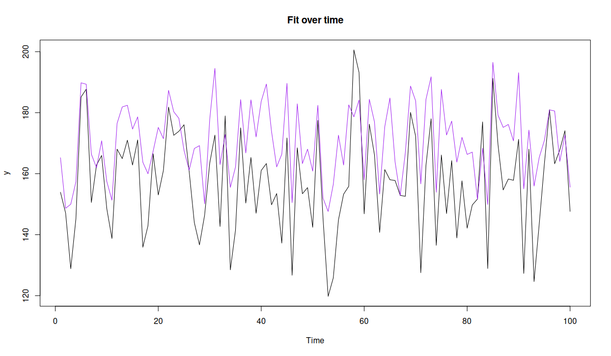
Dynamics of orders from alm model
The purple line in the Figure above corresponds to the orders and would cover roughly 90.91% of cases, so that we would run out of product in approximately 10% of cases, which would still be more profitable than any other option.
Finally, the approach works also well in case of non-linear newsvendor problem (see the paper for details), where quantile regression is not suitable and the conventional approach fails. The only thing that would change is the loss function, where the prices and costs would depend non-linearly on the order quantity and sales.
You can read the published paper on EJOR website or the working paper on ResearchGate.