


In one of the previous posts, we have discussed how to measure the accuracy of forecasting methods on the continuous data. All these MAE, RMSE, MASE, RMSSE, rMAE, rRMSE and other measures can give you an information about the mean or median performance of forecasting methods. We have also discussed how to measure the performance of models in terms of prediction intervals, and should now be comfortable with such measures as Range, Coverage, pinball, MIS. But all of this might become irrelevant when we face the intermittent demand – it can really make a bright day dark and screw with you and your measures. So, care is needed if you have data with randomly occurring zeroes.
We have already discussed aspects of intermittent demand in a post about the intermittent exponential smoothing model some time ago, and we have seen some time series examples in one of the previous posts, so I will not repeat myself, but I still think that there are a couple of important notes worth making about it.
Intermittent time series is the series that has non-zero values occurring at irregular intervals. This implies that there might be some periods of time, when we observe zeroes (e.g. no one buys our product). An example of such time series is shown below:
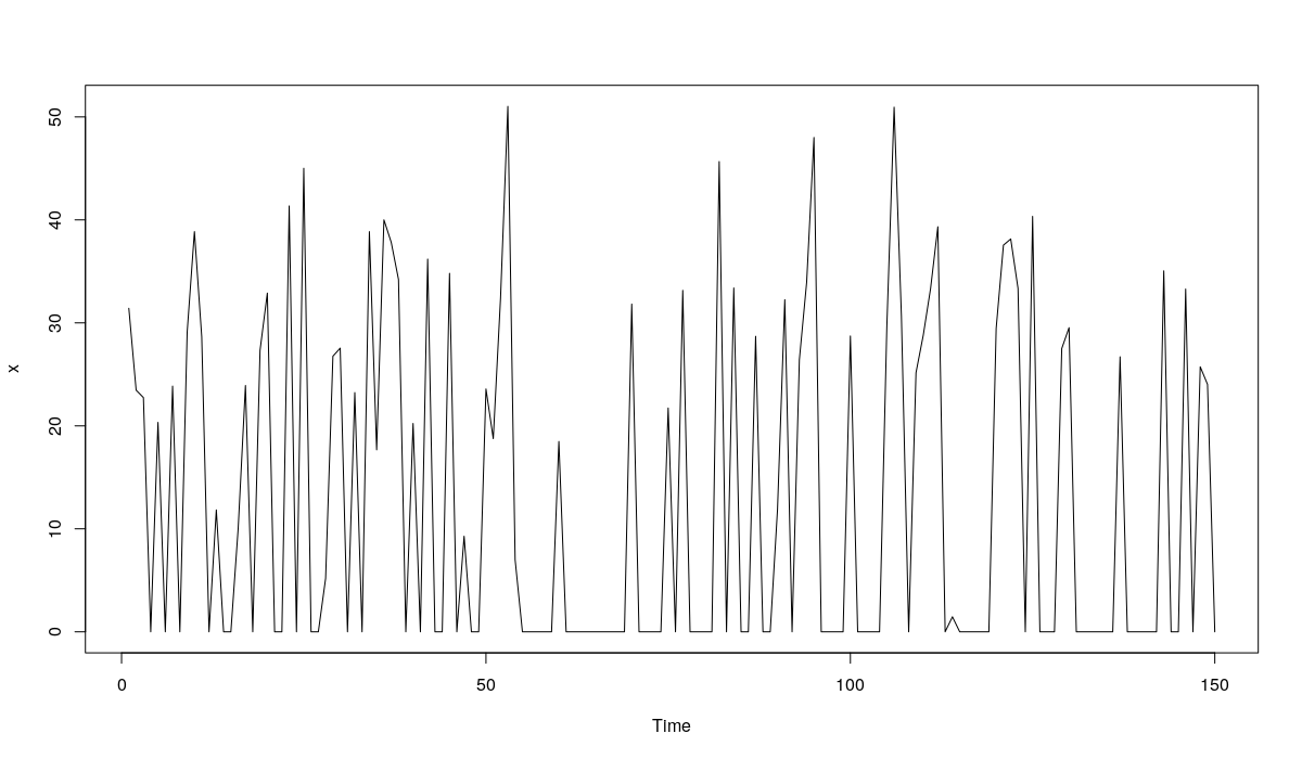
Intermittent Demand
As you can see, there are two sources of randomness in this data: there is a randomness about the non-zero value itself (e.g. demand size) and there is also a randomness about the occurrence of the non-zero value (e.g. demand occurrence). So, a very general model for intermittent demand can be represented as:
\begin{equation} \label{eq:general}
y_t = o_t z_t ,
\end{equation}
where \(y_t\) is the observed value at time \(t\), \(o_t\) is the binary occurrence variable and \(z_t\) is the demand sizes variable. While there are some statistical models that don’t do this distinction, the intermittent demand forecasting methods that are most popular in practice do it either directly or indirectly.
Although we can create very fancy forecasting models (there are even tries to use neural networks for this), we usually cannot accurately predict, when specifically the product will be bought and how many units we will sell. All we usually can do is to produce the mean value and / or prediction intervals for the demand itself. And even if we do that, the next thing to ask ourselves is: “What do we do with that?”
In a supply chain context, the typical decision would be how many units of product to order or to produce, given the amount that we already have. In this case we are usually talking about the safety stock – how many units of the product we should hold, so that we satisfy the demand and don’t have empty shelves. Typically, this is determined based on calculation of quantiles of a distribution. In many cases, in practice, the Normal distribution is used, and I cannot describe on how many levels this is wrong (the most obvious thing to point out is that usually we cannot have negative amounts of product). But let’s not get too much distracted.
What does the safety stock typically depend on? In many cases this is not just the demand of a product, but specifically the demand over the lead time – for example, how many products we will sell over the next week. Why? Because the deliveries tend to happen once over a time period, e.g. once a week, and we tend to order products once in a period of time – it does not make sense to order the product each time we run out of it. So, we do periodic reviews of the inventory and decide, how much we should order, so that we don’t run out of stock until the next replenishment.
Good. So, how do we get the information about the demand over the lead time? Here comes our forecasting model! But all of this implies that we should focus not just on the point and interval forecasts for each specific horizon, but on the values aggregated over the lead time. This is the first important difference between conventional forecasting and forecasting for inventory purposes (see for example, Kourentzes et al., 2019).
As you can see, the relation between the actual demand forecast and the decision of how much to order is complex. And this means that all those nice error measures, discussed in the previous posts, might not give us the important information of how our model performs in terms of orders. The model can produce very accurate forecasts, but this does not necessarily translate directly to correct ordering policy.
In order to align the model with the specific decisions, one can revert to simulations, so that it becomes more apparent how the model performs in terms of achieved service level, lost sales and excess inventory (which all are sort of proxies to the object of real interest in practice – the cost). This is one of the common approaches in the modern supply chain and inventory literature. Unfortunately, this approach is computationally expensive and may vary from one situation to another, so you would need to set up the simulation for each separate company and potentially for different products.
An alternative approach would be to at least asses the performance of models over the lead time, not on each observation. This means that we need to refer to cumulative values over the period of time:
\begin{equation} \label{eq:demandOverTheLeadTime}
Y_{t+h} = \sum_{j=1}^h {y}_{t+j} .
\end{equation}
Then we can measure, for example, how our models perform in terms of working stock (aka “cycle stock”). In this case we are only interested in the mean demand over the lead time, which for the additive models is relatively easy to deal with because the expectation of the sum of the demands is equal to the sum of the expectations:
\begin{equation}
\begin{aligned}
\text{E} \left(\sum_{j=1}^h {y}_{t+j} \right) = & \text{E}\left(\sum_{j=1}^h (\hat{y}_{t+j}+e_{t+j})\right) =\\
&\sum_{j=1}^h \text{E}(\hat{y}_{t+j}) + \sum_{j=1}^h \text{E}(e_{t+j}) = \sum_{j=1}^h \text{E}(\hat{y}_{t+j}).
\end{aligned} \label{eq:workingStock}
\end{equation}
where \(\hat{y}_{t+j}\) is the point forecast of a model. This means that we can produce the \(h\) steps ahead forecast and aggregate it over the lead time \(h\) and then compare it with the actual values for the same period. However, if we deal with the additive models in this context, then we are assuming that the demand can be negative – which is usually unrealistic, especially for intermittent demand. This means that a different model is needed, and \eqref{eq:workingStock} might not hold any more. So, for example, in case of ETS(M,N,N) simulations are necessary in order to produce the correct cumulative conditional expectation over the lead time.
Now, let’s say that we have managed to produce meaningful cumulative point forecast. What’s the next step? We need to measure its accuracy. The good news is, RMSE-based measures can be used in order to assess the performance of models in terms of the working stock (I hope you still remember, why MAE- and MAPE-based measures are not appropriate for intermittent demand). So, we can evaluate the Squared Cumulative Error and compare models based on it:
\begin{equation} \label{eq:workingStockRMSCE}
\text{SCE} = \left( \sum_{j=1}^h y_{t+j} -\sum_{j=1}^h \hat{y}_{t+j} \right)^2 .
\end{equation}
We can use relative or scaled measures, if we want to compare performance of models across products – all the things discussed in the previous post are applicable here. The main limitation here is that, given that we deal with intermittent demand, Naive method might cause problems if used as a benchmark. An example is a situation, when it produces zero forecasts for the holdout sample (because the last observation was zero), and the holdout contains only zeroes. This might happen by chance, but it will mess your beautiful relative error measures. A simple average of the whole series might be more appropriate as a benchmark for the intermittent demand.
There is a measure, which is ideologically close to the SCE. It is called “Periods-In-Stock” – PIS (Walstrom, 2010):
\begin{equation} \label{eq:workingStockPIS}
\text{PIS} = \sum_{j=1}^h \hat{y}_{t+j} -\sum_{j=1}^h y_{t+j} .
\end{equation}
Have you noticed that it is calculated as forecast minus the actual values? This was done by the author intentionally, so that the sign of the measure aligns with the inventory decisions. If the value is negative, then this means that we missed sales. If it is positive, then this means that we had too much stock and did not sell as much as we should have. Petropoulos & Kourentzes (2015) have proposed several modifications of PIS, which allow aggregating this measure over several products. So, have a look at the paper if you are interested, but I will not expand here.
By looking at those error measures, we can evaluate the performance in terms of working stock. But, as it was mentioned before, this does not necessarily translate to safety stock performance. So we need to figure out how to align our error measures with it. It seems that the closest we can get to it is by producing the specific quantiles for the values accumulated over the lead time. We typically don’t care about the lower bound, because in case of intermittent demand it is usually just zero, plus, the lower bound is not helpful for inventory decisions (e.g., knowing what will be the level of sales in 2.5% of cases is not helpful). So, we are more interested in the upper bound. In a realistic situation we would need to simulate the data from our model (something like a 1000 runs for the possible future outcomes), sum it up over the lead time and then take the upper quantile (for example, 95% or 99%). We have to do it this way, because we might not have expressions for the quantiles for the values accumulated over the lead time. But this way we will get quite close to the safety stock.
How do we measure performance of models in terms of this upper bound? I would be inclined to recommend pinball function, keeping in mind its limitations, discussed in the previous post. We can also analyse the coverage and range, and if we really need to use something like Mean Interval Score (MIS), then it makes sense to use Quantile Score instead (Gneiting, 2007), because it only takes the upper bound into account. However it needs to be modified in order to reflect the idea of cumulative values:
\begin{equation} \label{QS}
\text{QS} = \left(Y_{t+h} – U_{t+h} \right) \left(\mathbb{1} \left\{ Y_{t+h} \leq U_{t+h} \right\} -\alpha \right) ,
\end{equation}
where \(\alpha\) is the confidence level (in our example 95% or 99%), \(U_{t+h}\) is the value of the quantile and \(\mathbb{1}(\cdot)\) is the indicator function, returning one, when the condition is true and zero otherwise. The QS has similar interpretation and working principle as MIS: if the values lie below the specified quantile, then the measure is penalised less than in the case, when they lie above: in the former case the indicator function returns 1, so the weight becomes \(1-0.95=0.05\), while in the latter case it is equal to zero, so the weight is \(0 -0.05 = -0.05\). Note also that in that latter case the difference between the actual value and the bound is negative. This means that QS will always be positive, and in the ideal situation, when all the future values lie on the bound, the QS is equal to zero. The difference between QS and pinball function is in what specifically they measure. The QS measures the performance in terms of coverage and range for the bound, while the pinball tries to measure, how accurately we hit the specific quantile. So, arguably, QS is closer to what we would be interested in real life: we want to have the coverage closer to nominal (so that we achieve the nominal service level), but with the smallest range possible (so that we do not order too much and do not have huge holding costs). Based on QS, we can calculate scaled or relative measures in order to compare performance of forecasting models across the products.
So, what about the other intermittent demand contexts? In some of them the situation might be quite different and in some sense easier than in supply chain. For example, in case of the forecasting the patients flow in a hospital, we often do not need to deal with values over the lead time, which simplifies things substantially. In addition, we might not care much about the average number of patients for a specific day, but be more interested in the prediction interval. This way we can assess how many patients to expect in the “worst” / “best” case scenarios for the selected confidence level. Based on these values, we then decide, how many nurses, doctors and beds we should have for a specific day in order to service, let’s say, 95% of the patients in the next 4 hours. Note that yet again the prediction interval is not directly related to this goal, but at least it can be considered as an approximation to it, if we know how many nurse and doctor hours we typically need in order to process a specific type of patient. This also implies that we should evaluate the accuracy of the prediction intervals, not the accuracy of the mean. And, when doing all of that in case of intermittent demand, once again, we usually don’t care about the lower bound, because we can typically say even without any model that in the worst (best?) case we won’t have any patients at all. Instead, we should concentrate on the upper bound of the prediction interval, and we can use the measures, discussed in the previous context in this post.
Having said all this, the general recommendation for dealing with intermittent demand – avoid it at all costs. Why? Because intermittent demand is messy to identify and to deal with. Besides, are you sure that you really need to produce forecasts on that level of sales? What specific decisions do you make based on those forecasts? Maybe you don’t need to know how many watermellons you will sell in each separate shop every day. Maybe you should switch to weekly data, where the intermittency disappears, or aggregate sales of products over larger volumes and over several shops in the chain… So, before diving into the problem and trying to evaluate models, think about the decisions you usually make based on those models.
If the frequency of obtaining zero MAEs is too high, you can use this approach (page 23):
https://www.researchgate.net/publication/282136084_Measuring_Forecasting_Accuracy_Problems_and_Recommendations_by_the_Example_of_SKU-Level_Judgmental_Adjustments
Dear Andrey Davydenko,
Yes, trimming can be used indeed. But it is just a solution to the problem appearing in the measure naturally. The point in this post is not about how to fix relative measures, but how to avoid the problem all together: use averages instead of Naive.
Kind regards,
Ivan Svetunkov